Creating a Drop-Down List in a Cell
Suppose you have a report where users should only be able to enter particular values in a cell. You can create a dropdown menu to limit what they’re able to choose from. Using the example from this VLOOKUP, if you want to look up an employee’s salary, you should only be able to use correct names of employees and weed out types.
(Note: In the current post, the VLOOKUP for finding the employee’s salary has been updated to search based on the employee’s name instead of employee ID. The table array is now B1:C11 and the column index number is 2.)
Select the cell where you want the list. In this example, we’ll use H1, where we’ll select the employee’s name. In the ribbon, select go to the Data Tab and select Data – Data Validation.

Under Settings, in the Allow menu, select List.

Click your cursor into the Source field and highlight the cells with the values you want to choose from in the dropdown menu.
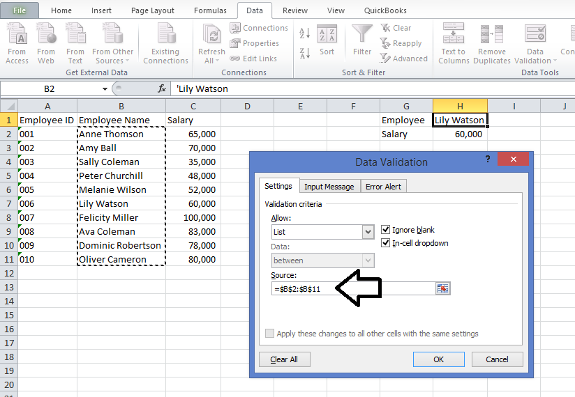
Click OK at the bottom of the popup window.

Now, when you select the cell, there will be a down arrow. If you click on that, you can choose options from the dropdown menu.

Entering an employee’s name will show you his or her salary.
 Using Drop-Down list in a cell it very nice comand and very usefull to us..
(Note: In the current post, the VLOOKUP for finding the employee’s salary has been updated to search based on the employee’s name instead of employee ID. The table array is now B1:C11 and the column index number is 2.)
Select the cell where you want the list. In this example, we’ll use H1, where we’ll select the employee’s name. In the ribbon, select go to the Data Tab and select Data – Data Validation.
Under Settings, in the Allow menu, select List.
Click your cursor into the Source field and highlight the cells with the values you want to choose from in the dropdown menu.
Click OK at the bottom of the popup window.
Now, when you select the cell, there will be a down arrow. If you click on that, you can choose options from the dropdown menu.
Entering an employee’s name will show you his or her salary.
Comments
Post a Comment