Posts

IF FUNCTION IN EXCEL

Image
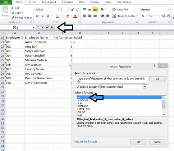
The IF function allows you to run a true-or-false test and return specific values based on the result. For example, if you’re doing annual employee reviews and whether each employee gets a raise is based on how well they’ve performed in the last year, you could run a yes-no test based on their score from their review. In this example, each employee’s performance is rated on a scale of 1 to 10. Any employee who scored a 6 or higher will get a raise. Select cell D21, then click on the fx button to get a window of available functions. Select IF and click OK.  The logical test is whether the performance score is equal to or greater than 6. The value if true is yes, and the value if false is no. If you only type in the words, Excel will automatically put in the quotation marks. Click OK, and copy the formula down for all employees. You can also nest multiple IF functions in each other. There are a couple downsides to this, such as they are difficult to maintain and troubl

Creating a Drop-Down List in a Cell

Image
Suppose you have a report where users should only be able to enter particular values in a cell. You can create a dropdown menu to limit what they’re able to choose from. Using the example from this VLOOKUP , if you want to look up an employee’s salary, you should only be able to use correct names of employees and weed out types. (Note: In the current post, the VLOOKUP for finding the employee’s salary has been updated to search based on the employee’s name instead of employee ID. The table array is now B1:C11 and the column index number is 2.)  Select the cell where you want the list. In this example, we’ll use H1, where we’ll select the employee’s name. In the ribbon, select go to the Data Tab and select Data – Data Validation. Under Settings, in the Allow menu, select List.    Click your cursor into the Source field and highlight the cells with the values you want to choose from in the dropdown menu.   Click OK at the bottom of the popup window. Now, when y

How to Hide Formula in Excel

Image
To hide formulas follow these simple steps: Step1: Un-Protect Worksheet At this point when you click on a cell, it shows you the entire formula in the formula bar. First of all, you need to make sure that your worksheet in unprotected. For this, go to review tab and in protect the group. If you find a “Unprotect Worksheet” button there, that means your worksheet is protected and you need to unprotect it. Click on that button to un protect it. If you have “Protect Sheet” button there that means your worksheet is unprotected. In that case, skip above steps and start from here. Step2: Activate Hide Formula Option Now, select the cell or range of cell, or select all the non-contiguous cells where you want to hide formulas. After that, right-click and select format cells option.      From format cells option, go to protection tab. In protection tab, you have two check boxes to mark, first locked and second is hidden. Mark on both

How to Remove Spaces in Excel

Image
In this tutorial, I will show you two ways to remove spaces in Excel. 1. Using TRIM function. 2. Using Find and Replace. #1 Using TRIM Function  excelentp.blogspot.in Excel TRIM function removes the leading and trailing spaces, and double spaces between text strings. For example, in the above example, to remove spaces from the entire list if first names (in A2:A7), use the following formula in cell C1 and drag it down for all the first names: =TRIM(A2) Excel TRIM function would instantly remove all the leading and trailing spaces in the cell. Once you have the cleaned data, copy it paste it as values in place of the original Data. This function is also helpful if you have more than one space character between words.It would remove the extra spaces such that the result always have one space character between words. Excel TRIM function does a good job in removing spaces in Excel, however, it fails when you have non-printing characters (such as lin

Delete Blank Rows in Excel

Image
Using Go To Special Technique to Delete Blank Rows in Excel Suppose you have a dataset as shown below: The above data has three blank rows in it.Here are the steps to quickly delete blank rows from this dataset.  Select the entire dataset (A1:C13 in this case).Press the F5 key It will open the Go To dialog box. You can get this dialog box from Home –> Editing –> Find and Select –> Go To. In the Go To dialog box, click on the Special button. This will open the Go To Special dialog box. In the Go To Special dialog box, select Blanks. Click Ok. This would select all the blank cells in the dataset.  Now that you have all the blank rows selected, here are the steps to delete these rows: Right-click on any of the selected cells and select Delete. In the Delete dialog box, select ‘Entire row’.   Click OK. This would instantly delete all the blank rows in the dataset. Note tha

How to Insert Bullet Points In Excel

Image
 1. Add a Bullet Point from Symbol Dialog BoxI bet you have used this method before. # Select the cell in which you want to add a bullet point. # Go to Insert Tab ► Click on Symbol.     #. Once you click on the symbol button, you’ll get a symbol dialog box.     #. In symbol dialog box, you have a lot of smart symbols to use as a bullet point or you can simply         use a black dot.     #. Once you choose your bullet point, just click on the insert to add in the cell. Here are some symbols which you can use as a bullet point. 2. Insert Bullet Points with a Shortcut Key Shortcut keys are the best way to insert a bullet point if you don’t have the time to play with symbol dialog box. We have two different shortcut keys and you can use any of these.  # Select the cell in which you want to add a bullet point.   Press F2 to edit cell.  Hold alt key and press 7 or 9 to insert a bullet.  Both shortcuts keys will give you a

How to Automatically Add Serial Numbers in Excel

Image
Serial numbers are like salt. You never feel their presence but their absence makes your data tasteless. Yes, they are important because, with a serial number, you can have a unique identity to each entry of your data. But the sad news is, adding them manually is a pain. It’s really hard to add a number in every row one after another.  The good news is, there are some ways which we can use to automatically add serial numbers in a column. 5 Ways to Insert Serial Number Column in Excel  And today, in this post, I’d like to share with you 5-Quick Methods. You can use any of these methods which you think is perfect for you. These methods can generate numbers up to a specific number or can add a running column of numbers. So without further ado, here are the methods. #1. Row Numbers as Serial Numbers. By default, in a spreadsheet, you have row numbers which act as a serial number for the date.If you don’t want to use serial numbers for filtering or any other purpose then